BP(back propagation)神经网络是1986年由Rumelhart和McClelland为首的科学家提出的概念，是一种按照误差逆向传播算法训练的多层前馈神经网络，是目前应用中最基本的神经网络。

运行环境：tensorflow1.14.0

新建程序文件

打开ide

我这里使用的是jupyter notebook，优点是容易调试，简单清爽。

在终端输入jupyter notebook即可在浏览器里面打开，windows是在cmd里面输入。

载入必要的库

# 第一步：引入库
import tensorflow as tf
import numpy as np
import matplotlib.pyplot as plt
%matplotlib inline
from skimage.io import imread
from skimage.transform import resize
import os
import random

载入封装好的函数

封装生成参数函数，全连接层函数等

# 第二步：封装卷积函数等
def weight_variable(shape):    
    initial = tf.truncated_normal(shape, mean=0, stddev=0.01)
    #正态初始化    
    return tf.Variable(initial)

def bias_variable(shape):    
    initial = tf.constant(0.1, shape=shape)    
    return tf.Variable(initial)

def fulc(x,next_depth):    
    depth = x.get_shape()[-1].value    
    w = weight_variable([depth, next_depth])    
    b = bias_variable([next_depth])    
    r = tf.nn.relu(tf.nn.bias_add(tf.matmul(x, w), b))    
    return r

封装读取图片函数（顺便给标签）

# 第三步：封装读取图片并自动给标签函数
def load_images(path):    
    contents = os.listdir(path)    
    classes = [each for each in contents if os.path.isdir(os.path.join(path,each))]    
    print('目录下有%s' % classes)        
    # 用labels来存储图片的类别    
    labels = []    
    # images数组用来存储图片数据   
    images = []    
    # 对每个不同种类读取图片到list并且+标签    
    for each in classes:        
        class_path = os.path.join(path,each)        
        files = os.listdir(class_path)        
        print("Starting {} images".format(each),'数量为',len(files))        
        for ii, file in enumerate(files, 1):            
            # 载入图片并放入batch数组中            
            img = imread(os.path.join(class_path, file))            
            img = img / 255.0         
            img = resize(img, (32, 32))           
            images.append(img.reshape((32,32,3)))            
            labels.append(each)   
	images = np.array(images)   
	#将labels的list形式转换为one_hot_label   
	from sklearn.preprocessing import LabelBinarizer  
    lb = LabelBinarizer()   
    lb.fit(labels)   
    labels_vecs = lb.transform(labels)   
    print('总共读取了%d张图片'%images.shape[0])  
    # print(labels,labels_vecs)  
    return images,labels_vecs # 返回图片以及对应的标签

随机抽取图片并打乱顺序

def next_batch(train_data, train_target, batch_size): #抽取数据   
    index = [ i for i in range(0,len(train_data))]      
    np.random.shuffle(index);   
    batch_data = np.zeros((batch_size,train_data.shape[1],train_data.shape[2],train_data.shape[3]));  
    batch_target = np.zeros((batch_size,train_target.shape[1]));   
    rand = random.randint(1,4)*2   
    for i in range(0,batch_size):      
        batch_data[i,:,:,:] = train_data[index[i],:,:,:]       
        #rotate(train_data[index[i]],rand,height,width)        
        batch_target[i,:] = train_target[index[i],:]  
    state = np.random.get_state()    
    np.random.shuffle(batch_data)  
    np.random.set_state(state)   
    np.random.shuffle(batch_target)  
    return batch_data, batch_target

封装神经网络结构

把上面的封装好的函数拿来用。

# 第四步：封装神经网络的创建函数
def create(x_images,keep_prob):#x_images的shape是h,w,d    
    h,w,d=x_images.get_shape().value    
    #first fully layer   
    h_conv_flat = tf.reshape(x_images,[-1,h*w*d])  
    h_fc1 = fulc(h_conv_flat,1024)   
    h_fc1_drop = tf.nn.dropout(h_fc1, keep_prob) 
    #second fully layer   
    h_fc2 = fulc(h_fc1_drop,1024)  
    h_fc2_drop = tf.nn.dropout(h_fc2, keep_prob)     
    #third full layer  
    h_fc3 = fulc(h_fc2_drop,1) 
    out = tf.nn.sigmoid(h_fc3,name='out')  
    # 二分类（输出为1个数字）可以用sigmoid；多分类用softmax      
    print('模型建立好了！')   
    return out

tensorflow特色占位

在tensorflow1.x版本内，训练前需要先在内存中“占位”。

既然如此，我们把模型创建、损失函数的定义、准确率的定义也放到这一块。

# 占位
x_images = tf.placeholder(tf.float32,[None,32,32,3],name='x_images')
y = tf.placeholder(tf.float32,[None,1],name='y')
keep_prob = tf.placeholder(tf.float32,name='keep_prob')

# 模型创建
y_conv = create(x_images,keep_prob)
# 定义损失函数、预测函数和训练过程
pred = tf.round(y_conv,name='predict')
cross_entropy = tf.reduce_mean(tf.reduce_mean(tf.square(y_conv-y)),name='cross_entropy')
train_step = tf.compat.v1.train.AdamOptimizer(1e-4).minimize(cross_entropy)

# 多分类定义准确率
# correct_prediction = tf.equal(tf.argmax(pred,1),tf.argmax(y,1))
# correct_prediction = tf.cast(correct_prediction, tf.float32)
# accuracy = tf.reduce_mean(correct_prediction,name='accuracy')

# 二分类定义准确率
correct_prediction = tf.equal(pred,y)
correct_prediction = tf.cast(correct_prediction, tf.float32)
accuracy = tf.reduce_mean(correct_prediction,name='accuracy')

开始训练

训练目标：训练集{batch_x,batch_y}100%正确

训练集：从{train_x，train_y}中抽取20对

每10次迭代打印并记录一次loss&acc值

saver = tf.compat.v1.train.Saver()
# 为保存模型做准备
with tf.Session() as sess:    
    sess.run(tf.compat.v1.global_variables_initializer())  
    step = 1   
    acc=0    
    while acc!=1:# 正确率达到100%才结束训练    
        batch_x,batch_y = next_batch(train_x,train_y,20)       
        # print(batch_y)   
        _ = sess.run(train_step,feed_dict={x_images: batch_x, y: batch_y, keep_prob: 0.75})     
        if step % 10 == 0:
            predt,acc,loss=sess.run([pred,accuracy,cross_entropy],feed_dict={x_images: batch_x, y: batch_y, keep_prob: 1.})
            print ('step:%d,train loss:%f' % (step,loss))             
            print('train accuracy:%f' % acc)                
            # 把训练损失的变化记录到本地，以便于以后的查阅     
            with open("trainloss.txt","a+") as f:               
                f.write('step:%d,train loss:%f\n' % (step,loss))                     
			# ---下面这个部分是为了接下来的误差、准确率的可视化---    
            if step==10:         
                l = np.array(loss)     
                a = np.array(acc)       
                s = np.array(step)    
			else:      
                l = np.append(l,np.array(loss))        
                a = np.append(a,np.array(acc))         
                s = np.append(s,np.array(step))     
                # ---结束可视化数据的收集---   
		step += 1   
        saver.save(sess,"./model/net.ckpt")# 当训练完成，把参数保存下来

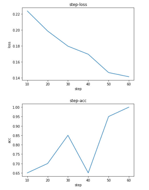
训练过程的可视化

使用以下代码

plt.plot(s,l)plt.title('step-loss')
plt.xlabel('step')
plt.ylabel('loss')
plt.show()
# -------loss&&acc---------
plt.plot(s,a)
plt.title('step-acc')
plt.xlabel('step')
plt.ylabel('acc')
plt.show()

效果如图：

最后：

本次实验中训练次数较少，且没有设置测试集或验证集，因此仅能作为参考，具体项目切不可如此。

猪老大要进步！

TensorFlow 1.x 实战--训练BP神经网络